线性回归模型

线性回归（Linear Regression）属于统计学习中的经典回归模型，通常用于发现变量间的线性关系或对连续型变量值进行预测。通常所说的线性回归一般指最小二乘回归（Least-Squares Regression），即将最小化均方损失函数（Mean Squared Loss Function）作为模型拟合的目标，此类问题也称最小二乘问题。

相关系数

相关系数（Correlation Coefficient）用于衡量两个随机变量之间的线性关系的强度和方向。相关系数的绝对值越接近 \(1\)，说明随机变量之间的线性关系越强，越适合使用线性回归模型来拟合；反之越接近 \(0\) 则越弱。

$$\rho_{X,Y} = \frac{cov(X,Y)}{\sigma_X \sigma_Y}$$

其中 \(cov\) 表示协方差，\(\sigma_X\) 和 \(\sigma_Y\) 是标准差。

一般线性回归模型

$$y = w_1 \cdot x + w_0$$

其中 \(x\) 为输入特征向量（可以为高维向量），\(y\) 为输出变量（当由多个值组成时称为多元（Multi-Variate）线性回归），\(w_1\) 为权重矩阵，\(w_0\) 为纵轴上的截距（\(w\) 的大小适应 \(x\) 和 \(y\) ）。

损失函数

均方损失函数（Mean Squared Loss Function）

$$\mathcal{L}(w_1, w_0) = \frac{1}{N}\sum_i^N {[y_i – (w_1 x_i + w_0)]}^2$$

模型参数优化

目标：最小化均方损失函数。

对于该线性损失函数，即分别求 \(\mathcal{L}\) 关于 \(w_1\) 和 \(w_0\) 的偏导数等于 \(0\) 时， \(w_1\) 和 \(w_0\) 值。由于该方程为线性的二次方程形式，因此模型参数是可解的。

解：

$$\begin{align} w_1 &= \frac{\sum_{i=1}^N (x_i – \bar{x}) (y_i – \bar{y})}{\sum_{i=1}^N (x_i – \bar{x})^2}, \\ w_0 &= \bar{y} – w_1\bar{x} \end{align}$$

模型评估

均方损失/残差（Residual Variance）

$$\sigma_{res}^2 = \frac{1}{N}\sum_{i=1}^N {[y_i – \tilde{y}_i]}^2 $$

其中 \(\tilde{y}_i\) 为模型预测值，\(y_i\) 为对应的真实值。其值越接近 \(0\)，模型拟合的越好。

决定系数 \(R^2\)

$$R^2 = \frac{\sigma_{reg}^2}{\sigma_{tot}^2}$$

其值越接近 \(1\)，模型拟合的越好。

其中 \(\sigma_{tot}^2\) 为总方差（Total Variance），\(\sigma_{reg}^2\) 为回归方差（Regression Variance），计算公式如下：

$$\begin{align} \sigma_{tot}^2 &= \frac{1}{N} \sum_i^N (y_i – \bar{y})^2 \\ \sigma_{reg}^2 &= \frac{1}{N} \sum_i^N (\tilde{y}_i – \bar{y})^2 \end{align}$$

一般的，有

$$\sigma_{reg}^2 + \sigma_{res}^2 = \sigma_{tot}^2$$

多项式回归

有时，对于关系较为复杂的两个变量，普通的线性回归可能无法很好的进行拟合。这时，可以把模型拓展为多项式的形式进行拟合，称多项式回归（Polynomial Regression）。模型的复杂度即多项式的度数可以自行调节，该模型可视化后呈现为一条曲线。

$$y = w_0 + w_1 x + w_2 x^2 + \cdot \cdot \cdot + w_d x^d$$

对于度数为 \(d\) 的多项式，共有 \(d+1\) 个可调节的参数。

类似于线性回归，多项式回归同样可以采用均方损失函数进行模型的参数优化，且参数值同样可解。

多项式回归的特别之处在于其具有一个额外的超参数（Hyperparameter）\(d\)，决定模型的复杂度。超参数过大会导致过拟合（Over-fitting），反之会造成欠拟合（Under-fitting），在训练时一般通过验证集或不断手动调节来寻找最优的超参数。

sklearn实现

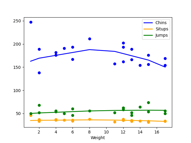
下面我采用sklearn的linnerud数据集，使用多元多项式回归探究体重与多个运动量之间的超线性关系。代码中包含了探索相关系数、划分数据集、模型的训练和预测、模型评估以及最终的可视化。

import numpy as np
from matplotlib import pyplot as plt
from sklearn.datasets import load_linnerud
from sklearn.model_selection import train_test_split
from sklearn.linear_model import LinearRegression
from sklearn.preprocessing import PolynomialFeatures
from sklearn.pipeline import make_pipeline

"""
Multivariate polynomial linear regression
Explore the relation between Weight and exercises (Chins, Situps and Jumps)
"""

# load data
X, y = load_linnerud(return_X_y=True)
X = X[:, [0]]

# explore correlations
print("Correlation Coefficient")
print('Weight - Chins: ', np.corrcoef(X[:, 0], y[:, 0])[0, 1])
print('Weight - Situps: ', np.corrcoef(X[:, 0], y[:, 1])[0, 1])
print('Weight - Jumps: ', np.corrcoef(X[:, 0], y[:, 2])[0, 1])

# split dataset
X_train, X_test, y_train, y_test = train_test_split(X, y, test_size=0.4, random_state=0)

# train model and predict
pipeline = make_pipeline(PolynomialFeatures(2), LinearRegression())
pipeline.fit(X_train, y_train)
y_pred = pipeline.predict(X_test)

# evaluate accuracy
accuracy_score = pipeline.score(X_train, y_train)
print('\nModel Accuracy: ', accuracy_score)

# visualisation
results = [(X_test[i], y_pred[i]) for i in range(X_test.shape[0])]
results.sort(key=lambda x: x[0])
X_result = [m[0] for m in results]
y_result = np.array([m[1] for m in results])
plt.plot(X_result, y_result[:, 0], color='blue', linewidth=2, label='Chins')
plt.plot(X_result, y_result[:, 1], color='orange', linewidth=2, label='Situps')
plt.plot(X_result, y_result[:, 2], color='green', linewidth=2, label='Jumps')
plt.scatter(X, y[:, 0], color='blue')
plt.scatter(X, y[:, 1], color='orange')
plt.scatter(X, y[:, 2], color='green')
plt.xlabel('Weight')
plt.legend()
plt.show()

程序输出

Correlation Coefficient
Weight - Chins:  -0.38969365080345586
Weight - Situps:  -0.5522321318045051
Weight - Jumps:  0.15064801968361358 

Model Accuracy:  0.23820863009731993