使用kd树实现knn算法

KNN算法是将待测样本与训练样本的特征进行比较，取k个与待测样本最接近的训练样本（如计算欧氏距离），其中k个样本中大多数属于哪一类别便也将待测样本分类为哪一类别（最大分类决策）。

Kd树是高效的实现KNN算法的一种实现方式，其中的k代表有k个维度。

Kd树的每个节点都可以看做一颗子树，他们拥有一致的属性和方法，因此kd树的构造和搜索都以递归的方式进行。

首先构造节点类，每个节点都有根值、左孩子、右孩子三个基本属性。

class node:
    def __init__(self):
        #根节点
        self.root = None
        #左孩子
        self.left = None
        #右孩子
        self.right = None

然后开始构造kd树，struct函数需要传入数据集，树的高度和父节点。构造出的节点属性包括节点所在高度，节点对应的搜索数据的轴，父节点，节点值（第n轴排序得到的中位数所在节点），标签，左子树（由中位数左侧的数据递归构建）和右子树（由中位数右侧的数据递归构建）。

    def struct(self,x,height=0,father=None):
        #数据集维度
        dimension = x.shape[1] - 1
        #节点高度
        self.height = height
        #节点对应的轴
        self.axis = self.height % dimension
        #父节点
        self.father = father
        
        #按第axis轴排序
        x = np.array(sorted(x,key=lambda a:a[self.axis]))
        #选取中位数作为切分点
        median = x.shape[0] // 2
        #根节点保存数据
        self.root = x[median][:-1]
        #保存数据标签
        self.target = int(x[median][-1])
        
        #递归构建kd树，其中若一侧无剩余元素，则对应孩子为None
        if x[:median].shape[0]:
            self.left = node()
            self.left.struct(x[:median],height=self.height+1,father=self)
        else:
            self.left = None
        
        if x[median+1:].shape[0]:
            self.right = node()
            self.right.struct(x[median+1:],height=self.height+1,father=self)
        else:
            self.right = None

这样，一棵kd树便递归的构造完成了，通过每个节点的root属性访问节点的数据值，left属性访问左节点，right属性访问右节点。

下面开始搜索kd树。

首先以最近邻为例进行搜索。

用特定变量来保存搜索到的当前最近点和根节点，保存的根节点用于之后判断是否搜索到了树顶。

    def search(self,x):
        #保存当前最近点
        current_nearest = None

        #保存根节点
        rootest_node = self

搜索第一步：递归向下搜索，在每一层的节点对应的轴的数值上进行比较，若目标点小于节点值，则进入左子树，反之进入右子树，直到到达叶节点，将该叶节点保存为当前最近点。

        #递归向下找到首个当前最近叶子节点
        def downward(check_node=self):
            #若到达叶子节点，则退出
            if check_node.left == None and check_node.right == None:
                return check_node
            
            #比较第axis轴元素，分别进入左右子树，其中若子树为空，则自动进入另外一子树
            if x[check_node.axis] < check_node.root[check_node.axis]:
                if check_node.left:
                    return downward(check_node.left)
                else:
                    return downward(check_node.right)
            else:
                if check_node.right:
                    return downward(check_node.right)
                else:
                    return downward(check_node.left)
        
        #保存首个当前最近点
        current_nearest = downward()

到达底部节点后，开始向上递归查找。其中，若到达顶部根节点，则结束查找并退出。过程中首先判断父节点是否为当前最近点，判断方法是分别计算父节点和当前最近点与目标节点的欧式距离。检查完父节点后，需要判断当前最近点与目标节点形成的超圆是否与父节点的另一子节点区域相交（判断相交只需比较父节点所对应的轴到圆心的距离与超圆的半径），若不相交则继续递归的向上回退，若相交则在另一子区域递归的进行整个最近邻搜索过程，搜索结束后继续向上回退。

        #递归向上搜索最近点
        def upward(check_node,tmp_nearest=None):
            #当前最近点初始化
            if not tmp_nearest:
                tmp_nearest = check_node
            #保存检查过的子节点
            checked_node = check_node
            
            #若到达顶部根节点，则退出
            if check_node is rootest_node:
                return tmp_nearest
            
            #向上寻找父节点
            check_node = check_node.father
            
            #检查父节点是否为当前最近点
            if np.linalg.norm(check_node.root-x) < np.linalg.norm(tmp_nearest.root-x):
                tmp_nearest = check_node
                
            #判断另一子节点区域是否与超圆相交（利用父节点的第axis轴的值）
            if np.fabs(check_node.root[check_node.axis]-x[check_node.axis]) < np.linalg.norm(tmp_nearest.root-x):
                #判断是否有另一子节点，若为空，则返回父节点向上查询
                if check_node.left == None or check_node.right == None:
                    tmp_nearest = upward(checked_node.father,tmp_nearest)
                    return tmp_nearest

                #若相交，移动到另一子节点
                check_node = check_node.left
                if check_node is checked_node:
                    check_node = check_node.father.right
                
                #递归的进行最近邻搜索
                tmp2_nearest = check_node.search(x)
                #比较新老最近点
                if np.linalg.norm(tmp2_nearest.root-x) < np.linalg.norm(tmp_nearest.root-x):
                    tmp_nearest = tmp2_nearest
                
                #向上递归查找
                tmp_nearest = upward(check_node.father,tmp_nearest)
                
                #返回当前最近点
                return tmp_nearest
                

            else:
                #子区域与超圆不相交时，直接向上递归
                tmp_nearest = upward(check_node,tmp_nearest)
                #返回当前最近点
                return tmp_nearest
                
        #保存向上递归找到的当前最近点
        current_nearest = upward(current_nearest)
        #返回当前最近点
        return current_nearest

至此kd树的构造结束，下面开始进行实际的搜索。使用简单数据集进行验证：

#书上简单数据集
x = np.array([[2,3,0],[5,4,0],[9,6,0],[4,7,0],[8,1,0],[7,2,0]])
z = np.array([6,5])

这里数据实际上是二维数据，在每个数据后加0是为了兼容之后使用的鸢尾花有标签数据，即最后一项作为标签项。待测数据选取（6，5）坐标点。

运行代码：

kdTree = node()
kdTree.struct(x)
result = kdTree.search(z)

print(result.target,result.root)

结果如下：

0 [5 4]

可见，结果将其标签分类为0（因为所有数据都是第0类），最近邻点是（5，4），答案正确。

使用鸢尾花数据集进行验证：

#将标签压入数据集，作为最后一个值
iris = load_iris()
x = iris.data  #数据
y = iris.target #标签
y = y[np.newaxis,:].T
x = np.column_stack((x,y))
z = np.array([6,5,0,0])

结果如下：

0 [5.8 4.  1.2 0.2]

可见，四维数据（6，5，0，0）被分为第0类，其最近邻点如图，从数值上看十分接近，应该是正确的。

下面将最近邻拓展至K近邻。

K近邻在KD树的构造上完全相同，只是搜索时用列表保存K个最近邻点即可，需要修改的保存和更新列表的函数如下：

        #保存k个最近点
        nearest_list = []

        #加入元素，排序判断大小，更新列表
        def update_nearest_list(element):
            nearest_list.append(element)
            nearest_list.sort(key=lambda t:np.linalg.norm(t.root-x))
            if len(nearest_list) > k:
                nearest_list.pop()

将k值传入到搜索函数中，用上述函数替换掉最近邻中更新当前最近点的部分即可，完整代码不再给出。

输入简单数据集验证，其中添加了绘图函数，使结果更直观：

def simple_data(k):
    #书上数据集
    x = np.array([[2,3,0],[5,4,0],[9,6,0],[4,7,0],[8,1,0],[7,2,0]])
    z = np.array([[6,5],[8,2]])

    
    kdTree = node()
    kdTree.struct(x)

    #直接显示书上数据集分类结果
    for i in range(z.shape[0]):
        result = kdTree.search(z[i],k)
        for j in result:
            print(j.root,end=' ')
        print('\n')

    #书上数据画图
    plt.figure(figsize=(6, 6))    #画布大小
    plt.plot(x[:,0],x[:,1],'rx',label='train data')
    plt.plot(z[:,0],z[:,1],'bo',label='test data')
    plt.xlabel('x')
    plt.ylabel('y')
    plt.xticks(range(0,11))  #x坐标轴刻度
    plt.yticks(range(0,11))  #y坐标轴刻度
    plt.grid()  # 生成网格
    plt.legend()
    plt.show()

k = 5
simple_data(k)

取k=5，结果如下：

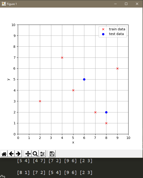
结果分别显示了（6，5）和（8，2）的5个近邻点。

使用鸢尾花数据集验证，其中将每一类50个数据中的30个作为训练数据，20个作为验证数据。

def iris_flower(k):

    #设置每一类训练数据数量
    num = 30

    #读取数据
    iris = load_iris()
    data = iris.data
    target = iris.target
    target_T = target[np.newaxis,:].T

    #训练数据（将标签压入数据集，作为最后一个值）
    x = np.row_stack((data[:num],data[50:50+num]))
    x = np.row_stack((x,data[100:100+num]))
    y = np.row_stack((target_T[:num],target_T[50:50+num]))
    y = np.row_stack((y,target_T[100:100+num]))
    x = np.column_stack((x,y))

    #无标签测试数据
    z = np.row_stack((data[num:50],data[50+num:100]))
    z = np.row_stack((z,data[100+num:150]))
    t = np.append(target[num:50],target[50+num:100])
    t = np.append(t,target[100+num:150])

    kdTree = node()
    kdTree.struct(x)

    #分类鸢尾花测试数据
    accurate = 0
    for j in range(z.shape[0]):
        result = kdTree.classify(z[j],k)
        if result == t[j]:
            accurate += 1
    print('正确率:',accurate/z.shape[0])

    #用鸢尾花前两维画图
    plt.plot(x[:num,0],x[:num,1],'rx',label='0')
    plt.plot(x[num:2*num,0],x[num:2*num,1],'bx',label='1')
    plt.plot(x[2*num:3*num,0],x[2*num:3*num,1],'yx',label='2')
    plt.xlabel('sepal length')
    plt.ylabel('sepal width')
    plt.legend()
plt.show()

k = 5时结果如下：

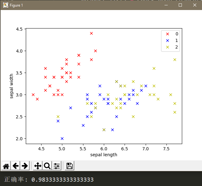
这里只是使用数据点的前两维绘图，可以看到第1类和第2类的数据错杂在了一起，以此可以看出只用前两维不能很好的区分这两类数据点。而算法中使用了全部的四维进行计算，最终的正确率还是十分可喜的。